Price Prediction Regression Model

Price prediction model

It was our end-semester project for our course on AI. We used the principles of machine learning to build a model that would be able to provide us with an optimal solution concerning the specific requirement of someone who requires to obtain the ticket.

Data set

The data set is an Indian data set taken from Kaggle. You can find it here.

EDA

Before using our data set to train the models we first have to clean our data. We first applied some EDA methods to our data set. Exploratory Data Analysis (EDA) is an approach to analyzing the data using visual techniques. It is used to discover trends, and patterns, or to check assumptions with the help of statistical summary and graphical representations. Our original data set shape was (20000, 11).

We removed the null values from our data set. Now the flight duration entry was given on a scale of 1 to 10. We converted this into a scale of 24 hrs. Then converted it into the panda’s date and time so that our model can handle these values more easily and efficiently.

Handling Categorical Data

All Machine Learning models are some kinds of a mathematical model that needs numbers to work with. Categorical data have possible values (categories) and it can be in text form. For example, Gender: Male/Female/Others, Ranks: 1st/2nd/3rd, etc

First, let’s understand the types of categorical data:

Nominal Data: The nominal data is called labeled/named data. Allowed to change the order of categories, change in order doesn’t affect its value. For example, Gender (Male/Female/Other), Age Groups (Young/Adult/Old), etc.
Ordinal Data: Represent discretely and ordered units. Same as nominal data but have ordered/rank. Not allowed to change the order of categories. For example, Ranks: 1st/2nd/3rd, Education: (High School/Undergrads/Postgrads/Doctorate), etc.

One Hot Encoding

Most of the columns in the data set were nominal data so we used one-hot encoding in our data set. One hot encoding is one method of converting data to prepare it for an algorithm and get a better prediction.

With one-hot, we convert each categorical value into a new categorical column and assign a binary value of 1 or 0 to those columns. Each integer value is represented as a binary vector. All the values are zero, and the index is marked with a 1.

While this is helpful for some ordinal situations, some input data does not have any ranking for category values, and this can lead to issues with predictions and poor performance. That’s when one hot encoding saves the day.

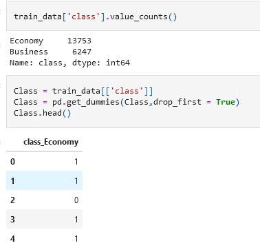
one hot encoding on “class” colums

The stops column was using ordinal data so we used simple number mapping for its encoding.

train\_data.replace({“one”:1, “zero”:0, “two\_or\_more”:2},inplace = True)

Now after applying the EDA methods our data-frame shape increased to (20000, 33). After done with the train data we also did the same with the test data with the final shape of (20000, 32).

Feature Importance

Now we did some feature extractions from our data set. Feature Importance refers to techniques that calculate a score for all the input features for a given model — the scores simply represent the “importance” of each feature. A higher score means that the specific feature will have a larger effect on the model that is being used to predict a certain variable

After feature extraction, we were able to see which features were playing the most important role in predicting the values

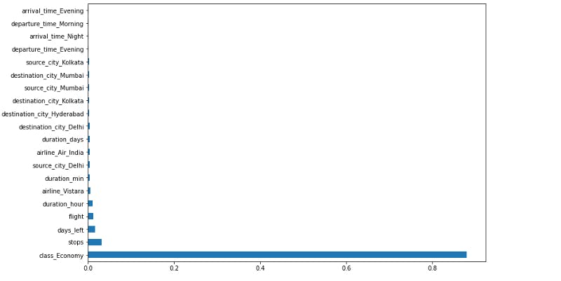
Graph showing that class-economy effecting the price most

Regression Models

Now we applied some regression models and calculated the score for each scenario.

Decision Tree Regressor
SVR
K-Neighbors Regressor
Elastic Net
Random Forest Regressor
Lasso
Linear Regression

from sklearn.linear_model import LinearRegression  
from sklearn.linear_model import Lasso  
from sklearn.ensemble import RandomForestRegressor  
from sklearn.linear_model import ElasticNet  
from sklearn.neighbors import KNeighborsRegressor  
from sklearn.svm import SVR  
from sklearn.tree import DecisionTreeRegressor  
from sklearn.model_selection import train_test_split  

X_train,X_test,y_train,y_test = train_test_split(X,y,test_size = 0.2,random_state = 1)  

models = []  

models.append(('LR', LinearRegression()))  
models.append(('LA', Lasso()))  
models.append(('RFR', RandomForestRegressor()))  
models.append(('EN', ElasticNet()))  
models.append(('KNN', KNeighborsRegressor()))  
models.append(('SVM', SVR()))  
models.append(('DTR', DecisionTreeRegressor()))  

names = []  
results = []  


for name, model in models:  
  model = model.fit(X_train, y_train)  
  accuracy = model.score(X_test,y_test)  
  results.append(accuracy)  
  names.append(name)  
  print('%s:%f'%(name, accuracy))

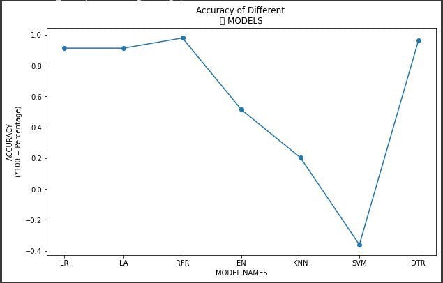
Random Forest gave the most score

Keeping in view the results we applied the random forest regression.

Applied random forest on the data

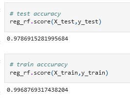
test and train score

Graph showing that how good was our model in predicting the values correctly

Hyper Parameters Tunning

We used the Randomized CV Search technique here. For random forest, we used the following parameters

# Number of trees in random forest

n_estimators = [int(x) for x in np.linspace(start = 100, stop = 1200, num = 12)]

# Number of features to consider at every split

max_features = [‘auto’, ‘sqrt’]

# Maximum number of levels in tree

max_depth = [int(x) for x in np.linspace(5, 30, num = 6)]

# Minimum number of samples required to split a node

min_samples_split = [2, 5, 10, 15, 100]

# Minimum number of samples required at each leaf node

min_samples_leaf = [1, 2, 5, 10]

After the processing, all the parameters the best parameters were found to be

{'n_estimators': 700,

'min_samples_split': 15,

'min_samples_leaf': 1,

'max_features': 'auto',

'max_depth': 20}

Now when we again trained our data using these parameters our score turns out to be 0.97706

You can find the whole source code here https://github.com/imranzaheer612/flight-fare-prediction-regression

Originally published at theundersurfers.netlify.app

Imran Zaheer